This function satisfies our requirements: It provides a way to move parameters in the desired direction, punishes unequal signs, and has zero loss if x and y have equal sign.
In summary: For a given pair of real vectors (each obtained by calculating the hash function without the last step of converting to a binary hash) we can simply sum the loss for each vector entry. We now have a loss function that we can use to adjust our parameters from examples.
Generating training data
Generating training data should - at least in theory - be simple. It should be sufficient to compile some open-source code with a number of different compilers and compiler settings, and then parse the symbol information to create groups of “function variants” - e.g. multiple different compiler outputs for the same C/C++ function. Similarly, known-dissimilar-pairs can be generated by simply taking two random functions with different symbols.
Unfortunately, theory is not practice, and a number of grimy implementation issues come up, mostly around symbol parsing and CFG reconstruction.
Real-world problems: Symbols
One problem arises from the non-availability of good cross-platform tooling for parsing different versions of the PDB file format - which naturally arise when many different versions of Visual Studio are used - and the difficulty of reliably building the same open-source codebase for many different compilers. While GCC and CLANG are often drop-in-replaceable, projects that build without intervention on both Visual Studio, GCC, and CLANG are much more rare.
The (unfortunate) solution to the PDB parsing issue is “giving up” - the codebase expects the PDB information to have been dumped to a text file. More on this below.
The (equally unfortunate) solution to the issue of building the same codebase reliably with Visual Studio and GCC is also “giving up” - it is up to the user of FunctionSimSearch to get things built.
Other problems arise by different mangling conventions for C++ code, and different conventions in different compilers affecting how exactly a function is named. This is solved by a hackish small tool that removes type information from symbols and tries to “unify” between GCC/CLANG and Visual Studio notation.
Real-world problems: Reliably generating CFGs, and polluted data sets
Obtaining CFGs for functions should be simple. In practice, none of the tested disassemblers correctly disassembles switch statements across different compilers and platforms: Functions get truncated, basic blocks mis-assigned etc. The results particularly dire for GCC binaries compiled using -fPIC of -fPIE, which, due to ASLR, is the default on modern Linux systems.
The net result is polluted training data and polluted search indices, leading to false positives, false negatives, and general frustration for the practitioner.
While the ideal fix would be more reliable disassembly, in practice the fix is careful investigation of extreme size discrepancies between functions that should be the same, and ensuring that training examples are compiled without PIC and PIE (-fno-pie -fno-PIE -fno-pic -fno-PIC is a useful set of build flags).
Data generation in practice
In practice, training data can be generated by doing:
cd ./testdata
./generate_training_data.py --work_directory=/mnt/training_data
The script parses all ELF and PE files it can find in the ./testdata/ELF and ./testdata/PE directories. For ELF files with DWARF debug information, it uses objdump to extract the names of the relevant functions. For PE files, I was unfortunately unable to find a good and reliable way of parsing a wide variety of PDB files from Linux. As a result, the script expects a text file with the format “<executable_filename>.debugdump” to be in the same directory as each PE executable. This text file is expected to contain the output of the DIA2Dump sample file that ships with Visual Studio.
The format of the generated data is as follows:
./extracted_symbols_<EXEID>.txt
./functions_<EXEID>.txt
./[training|validation]_data_[seen|unseen]/attract.txt
./[training|validation]_data_[seen|unseen]/repulse.txt
./[training|validation]_data_[seen|unseen]/functions.txt
Let’s walk through these files to understand what we are operating on:
The ./extracted_symbols_<EXEID>.txt files:
Every executable is assigned an executable ID - simply the first 64 bit of it’s SHA256. Each such file describes the functions in the executable for which symbols are available, in the format:
[exe ID] [exe path] [function address] [base64 encoded symbol] false
The ./functions_<EXEID>.txt files:
These files contain the hashes of the extracted features for each function in the executable in question. The format of these files is:
[exe ID]:[function address] [sequence of 128-bit hashes per feature]
The ./[training|validation]_data_[seen|unseen]/attract.txt and ./repulse.txt files:
These files contain pairs of functions that should repulse / attract, the format is simply
[exe ID]:[function address] [exe ID]:[function address]
The ./[training|validation]_data_[seen|unseen]/functions.txt files:
A file in the same format as the ./functions_<EXEID>.txt files with just the functions referenced in the corresponding attract.txt and repulse.txt.
Two ways of splitting the training / validation data
What are the mysterious training_data_seen and training_data_unseen directories? Why does the code generate multiple different training/validation splits? The reason for this is that there are two separate questions we are interested in:
Does the learning process improve our ability to detect variants of a function we have trained on?
Does the learning process improve our ability to detect variants of a function, even if no version of that function was available at training time?
While (2) would be desirable, it is unlikely that we can achieve this goal. For our purposes (detection of statically linked vulnerable libraries), we can probably live with (1). But in order to answer these questions meaningfully, we need to split our training and validation data differently.
If we wish to check for (2), we need to split our training and validation data along “function group” lines: A “function group” being a set of variant implementations of the same function. We then need to split off a few function groups, train on the others, and use the groups we split off to validate.
On the other hand, if we wish to check for (1), we need to split away random variants of functions, train on the remainder, and then see if we got better at detecting the split-off functions.
The differences in how the training data is split is best illustrated as follows:
 Implementation issues of the training
The industry-standard approaches for performing machine learning are libraries such as TensorFlow or specialized languages such as Julia with AutoDiff packages. These come with many advantages -- most importantly, automated parallelization and offloading of computation to your GPU.
Unfortunately, I am very stubborn -- I wanted to work in C++, and I wanted to keep the dependencies extremely limited; I also wanted to specify my loss function directly in C++. As a result, I chose to use a C++ library called SPII which allows a developer to take an arbitrary C++ function and minimize it. While this offers a very clean and nice programming model, the downside is “CPU-only” training. This works, but is uncomfortably slow, and should be replaced with a GPU-based version.
Running the actual training process
Once the training data is available, running the training process is pretty straightforward:
thomasdullien@machine-learning-training:~/sources/functionsimsearch/bin$ ./trainsimhashweights -data=/mnt/training_data/training_data_seen/ --weights=weights_seen.txt
[!] Parsing training data.
[!] Mapping functions.txt
[!] About to count the entire feature set.
[!] Parsed 1000 lines, saw 62601 features ...
[!] Parsed 2000 lines, saw 104280 features ...
(...)
[!] Parsed 12000 lines, saw 270579 features ...
[!] Processed 12268 lines, total features are 271653
[!] Iterating over input data for the 2nd time.
[!] Loaded 12268 functions (271653 unique features)
[!] Attraction-Set: 218460 pairs
[!] Repulsion-Set: 218460 pairs
[!] Training data parsed, beginning the training process.
Itr f deltaf max|g_i| alpha H0 rho
0 +7.121e+04 nan 4.981e+02 2.991e-06 1.000e+00 0.000e+00
1 +7.119e+04 2.142e+01 5.058e+02 1.000e+00 1.791e-06 3.114e-01
2 +7.101e+04 1.792e+02 3.188e+02 1.000e+00 2.608e-05 5.735e-03
3 +7.080e+04 2.087e+02 2.518e+02 1.000e+00 4.152e-05 4.237e-03
4 +7.057e+04 2.271e+02 2.757e+02 1.000e+00 5.517e-05 4.469e-03
...
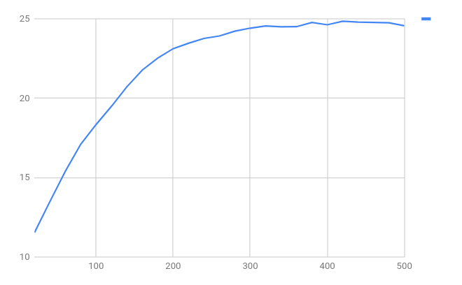
A few days later, the training process will have performed 500 iterations of L-BFGS while writing snapshots of the training results every 20 steps into our current directory (20.snapshot … 480.snapshot). We can evaluate the results of our training:
$ for i in *.snapshot; do foo=$(./evalsimhashweights --data /mnt/june2/validation_data_seen/ --weights $i | grep \(trained\)); echo $i $foo; done
This provides us with the “difference in average distance between similar and dissimilar pairs” in the validation data: the code calculates the average distance between similar pairs and between dissimilar pairs in the validation data, and shows us the difference between the two. If our training works, the difference should go up.
 We can see that somewhere around 420 training steps we begin to over-train - our difference-of-means on the validation set starts inching down again, so it is a good idea to stop the optimization process. We can also see that the difference-in-average-distance between the “similar” and “dissimilar” pairs has gone up from a bit more than 10 bits to almost 25 bits - this seems to imply that our training process is improving our ability to recognize variants of functions that we are training on.
Understanding the results of training
There are multiple ways of understanding the results of the training procedure:
Given that we can easily calculate distance matrices for a set of functions, and given that there are popular ways of visualizing high-dimensional distances (t-SNE and MDS), we can see the effects of our training visually.
Several performance metrics exist for information-retrieval tasks (Area-under-ROC-curve).
Nothing builds confidence like understanding what is going on, and since we obtain per-feature weights, we can manually inspect the feature weights and features to see what exactly the learning algorithm learnt.
The next sections will go through steps 1 and 2. For step 3, please refer to the documentation of the tool.
Using t-SNE as visualisation
A common method to visualize high-dimensional data from pairwise distances is t-SNE -- a method that ingests a matrix of distances and attempts to create a low-dimensional (2d or 3d) embedding of these points that attempts to respect distances. The code comes with a small Python script that can be used to visualize
We will create two search indices: One populated with the “learnt feature weights”, and one populated with the “unit feature weight”:
# Create and populate an index with the ELF unrar samples with the
# learnt features.
./createfunctionindex --index=learnt_features.index; ./growfunctionindex --index=learnt_features.index --size_to_grow=256; for i in $(ls ../testdata/ELF/unrar.5.5.3.builds/*); do echo $i; ./addfunctionstoindex --weights=420.snapshot --index=learnt_features.index --format=ELF --input=$i; done
# Add the PE files
for i in $(find ../testdata/PE/ -iname *.exe); do echo $i; ./addfunctionstoindex --weights=420.snapshot --index=learnt_features.index --format=PE --input=$i; done
# Create and populate an index with unit weight features.
./createfunctionindex --index=unit_features.index; ./growfunctionindex --index=unit_features.index --size_to_grow=256; for i in $(ls ../testdata/ELF/unrar.5.5.3.builds/*); do echo $i; ./addfunctionstoindex --index=unit_features.index --format=ELF --input=$i; done
# Add the PE files
for i in $(find ../testdata/PE/ -iname *.exe); do echo $i; ./addfunctionstoindex --index=unit_features.index --format=PE --input=$i; done
# Dump the contents of the search index into a text file.
./dumpfunctionindex --index=learnt_features.index > learnt_index.txt
./dumpfunctionindex --index=unit_features.index > unit_index.txt
# Process the training data to create a single text file with symbols for
# all functions in the index.
cat /mnt/training_data/extracted_*.txt > ./symbols.txt
# Generate the visualisation
cd ../testdata
./plot_function_groups.py ../bin/symbols.txt ../bin/learn_index.txt /tmp/learnt_features.html
./plot_function_groups.py ../bin/symbols.txt ../bin/learnt_index.txt /tmp/learnt_features.html
We now have two HTML files that use d3.js to render the results:
Unit weights:
Learned weights:
Mouse-over on a point will display the function symbol and file-of-origin. It is visible to the naked eye that our training had the effect of moving groups of functions “more closely together”.
We can see here that the training does have some effect, but does not produce the same good effect for all functions: Some functions seem to benefit much more from the training than others, and it remains to be investigated why this is the case.
Examining TPR, FPR, IRR, and the ROC-curve
When evaluating information retrieval systems, various metrics are important: The true positive rate (how many of the results we were supposed to find did we find?), the false positive rate (how many of the results we were not supposed to find did we find?), the irrelevant result rate (what percentage of the results we returned were irrelevant? This is the complement to the precision), and the ROC curve (a plot of the TPR against the FPR).
This is helpful in both making informed choices about the right distance threshold, but also in order to quantify how much we are losing by performing approximate vs. precise search. It also helps us choose how many "hash buckets" we want to use for approximate searching.
There is a Python script in the git repository that can be used to generate the data for the ROC curve. The script requires a file with the symbols for all elements of the search index, a textual representation of the search index (obtained with dumpsearchindex, and access to the actual search index file.
# Create a search index to work with.
./createfunctionindex --index=/media/thomasdullien/roc/search.index
# Make it big enough to contain the data we are adding.
./growfunctionindex --index=/media/thomasdullien/roc/search.index --size_to_grow=1024
# Add all the functions from our training directories to it:
for filename in $(find ../testdata/ELF/ -iname *.ELF); do echo $filename; ./addfunctionstoindex --format=ELF --input=$filename --index=/media/thomasdullien/roc/search.index; done
for filename in $(find ../testdata/PE/ -iname *.exe); do echo $filename; ./addfunctionstoindex --format=PE --input=$filename --index=/media/thomasdullien/roc/search.index; done
# Now dump the search index into textual form for the Python script:
./dumpfunctionindex --index /media/thomasdullien/roc/search.index > /media/thomasdullien/roc/search.index.txt
# The file "symbols.txt" is just a concatenation of the symbols extracted during
# the run of the ./generate_training_data.py script.
cat /media/thomasdullien/training_data/extracted_symbols_*.txt > /media/thomasdullien/roc/symbols.txt
In order to obtain the data for the curve, we can use the following Python script:
testdata/evaluate_ROC_curve.py --symbols=/media/thomasdullien/roc/symbols.txt --dbdump=/media/thomasdullien/roc/search.index.txt --index=/media/thomasdullien/roc/search.index
The output of the script is a 7-column output:
The maximum distance between two SimHash values to consider.
The true positive rate for exact (non-approximate-search-index) search.
The false positive rate for exact (non-approximate-search-index) search.
The true positive rate for search using the approximate search index.
The false positive rate for using the approximate search index.
The percentage of irrelevant results returned using exact search.
The percentage of irrelevant results returned using approximate search.
We can generate the curves for both the trained and untrained data, and then plot the results using gnuplot:
gnuplot -c ./testdata/plot_results_of_evaluate_ROC_curve.gnuplot ./untrained_roc.txt
gnuplot -c ./testdata/tpr_fpr_curve.gnuplot ./untrained_roc.txt ./trained_roc.txt
So let us examine this plots for the untrained results first:

The first diagram shows that if we want a TPR of more than 50%, we will have to incur about 20% of the returned results being irrelevant to our search; the cut-off distance we should take for this is somewhere around 25 bits.
We also see that we will pay a heavy price for increasing the cut-off: At 35 bits, where our TPR hits 55%, half of our results are irrelevant. This is a weakness of the set-up at the moment, and we will see if it can be improved by learning weights.
The second diagram shows that we only pay in TPR for the approximate search for very high cut-offs - the TPR and FPR flatten off, which is a symptom of us missing more and more of the search space as we expand the number of bits we consider relevant.
The lower-left diagram shows how quickly our precision deteriorates as we try to improve the recall.
How are these curves affected by the training process?

So in the top-left curve, we can see that the rate of irrelevant results at 10 bits distance has dropped significantly: Down to approximately 5% from about 15%. Unfortunately, the true-positive-rate has also dropped - instead of about 45% of the results we want to get, we only achieve about 33%. So the training works in the sense that it improves the ratio of good results to irrelevant results significantly, but at the cost of lowering the overall rate of results that we find.
If we are willing to tolerate approximately 15% irrelevant results, we will get about 45% of the results we desire in the non-trained version. Sadly, in the trained version, for the same level of irrelevant results, we only get about 40% of the results we desire.
In summary: In the current form, the training is useful for lowering the irrelevant result rate below what is achievable without training - but for any acceptable rate of irrelevant results that can be achieved without training, the untrained version appears to achieve better results.
Does this generalize to out-of-sample functions?
In the section about splitting our training/validation data, we posed two questions - and the more interesting question is (2). Is there anything we are learning about the compilers ?
Plotting the difference-in-mean-distance that we plotted for question (1) also for question (2) yields the following image:

The red curve implies that there is a faint but non-zero signal - after about 80 training steps we have increased the mean-difference-in-means from 11.42 bits to 12.81 bits; overtraining appears to begin shortly thereafter.
It is unclear how much signal could be extracted using more powerful models; the fact that our super-simple linear model extracts something is encouraging.
Practical searching
Using FunctionSimSearch from any Python-enabled RE tool
The command-line tools mostly rely on DynInst for disassembly - but reverse engineers work with a bewildering plethora of different tools: IDA, Radare, Binary Ninja, Miasm etc. etc.
Given the development effort to build integration for all these tools, I decided that the simplest thing would be to provide Python bindings -- so any tool that can interact with a Python interpreter can use FunctionSimSearch via the same API. In order to get the tool installed into your Python interpreter, run:
python ./setup.py --install user
The easiest way to use the API from python is via JSON-based descriptions of flowgraphs:
jsonstring = (... load the JSON ... )
fg = functionsimsearch.FlowgraphWithInstructions()
fg.from_json(jsonstring)
hasher = functionsimsearch.SimHasher("../testdata/weights.txt")
function_hash = hasher.calculate_hash(fg)
This yields a Python tuple with the hash of the function. The JSON graph format used as input looks as follows:
{
"edges": [ { "destination": 1518838580, "source": 1518838565 }, (...) ],
"name": "CFG",
"nodes": [
{
"address": 1518838565,
"instructions": [
{ "mnemonic": "xor", "operands": [ "EAX", "EAX" ] },
{ "mnemonic": "cmp", "operands": [ "[ECX + 4]", "EAX" ] },
{ "mnemonic": "jnle", "operands": [ "5a87a334" ] } ]
}, (...) ]
}
More details on how to use the Python API can be found in this example Python-based IDA Plugin. The plugin registers hotkeys to “save the current function in IDA into the hash database” and hotkeys to “search for similar functions to the current IDA function in the hash database”. It also provides hotkeys to save the entire IDB into the Database, and to try to match every single function in a given disassembly against the search index.
For people that prefer using Binary Ninja, a plugin with similar functionality is available (thanks carstein@ :-).
Searching for unrar code in mpengine.dll
As a first use case, we will use IDA to populate a search index with symbols from unrar, and then search through mpengine.dll (also from Binary Ninja) for any functions that we may recognize.
We can populate a search index called '''/var/tmp/ida2/simhash.index''' from a set of existing disassemblies using the following command line:
# Create the file for the search index.
/home/thomasdullien/Desktop/sources/functionsimsearch/bin/createfunctionindex --index=/var/tmp/ida2/simhash.index
# Populate using all 32-bit UnRAR.idb in a given directory.
for i in $(find /media/thomasdullien/unrar.4.2.4.builds.idbs/unrar/ -iname UnRAR.idb); do ./ida -S"/usr/local/google/home/thomasdullien/sources/functionsimsearch/pybindings/ida_example.py export /var/tmp/ida2/" $i; done
# Populate using all 64-bit UnRAR.i64 in a given directory.
for i in $(find /media/thomasdullien/unrar.4.2.4.builds.idbs/unrar/ -iname UnRAR.i64); do ./ida64 -S"/usr/local/google/home/thomasdullien/sources/functionsimsearch/pybindings/ida_example.py export /var/tmp/ida2/" $i; done
Once this is done, we can open mpengine.dll in IDA, go to File->Script File and load ida_example.py, then hit "Shift-M".
The IDA message window will get flooded with results like the text below:
(...)
6f4466b67afdbf73:5a6c8da1 f3f964313d8c559e-e6196c17e6c230b4 Result is 125.000000 - 72244a754ba4796d:42da24 x:\shared_win\library_sources\unrar\unrarsrc-4.2.4\unrar\build.VS2015\unrar32\Release\UnRAR.exe 'memcpy_s' (1 in inf searches)
6f4466b67afdbf73:5a6c8da1 f3f964313d8c559e-e6196c17e6c230b4 Result is 125.000000 - ce2a2aa885d1a212:428234 x:\shared_win\library_sources\unrar\unrarsrc-4.2.4\unrar\build.VS2015\unrar32\MinSize\UnRAR.exe 'memcpy_s' (1 in inf searches)
6f4466b67afdbf73:5a6c8da1 f3f964313d8c559e-e6196c17e6c230b4 Result is 125.000000 - 69c2ca5e6cb8a281:42da88 x:\shared_win\library_sources\unrar\unrarsrc-4.2.4\unrar\build.VS2015\unrar32\FullOpt\UnRAR.exe 'memcpy_s' (1 in inf searches)
--------------------------------------
6f4466b67afdbf73:5a6f7dee e6af83501a8eedd8-6cdba61793e9a840 Result is 108.000000 - ce2a2aa885d1a212:419301 x:\shared_win\library_sources\unrar\unrarsrc-4.2.4\unrar\build.VS2015\unrar32\MinSize\UnRAR.exe '?RestartModelRare@ModelPPM@@AAEXXZ' (1 in 12105083908.189119 searches)
6f4466b67afdbf73:5a6f7dee e6af83501a8eedd8-6cdba61793e9a840 Result is 107.000000 - 86bc6fc88e1453e8:41994b x:\shared_win\library_sources\unrar\unrarsrc-4.2.4\unrar\build.VS2013\unrar32\MinSize\UnRAR.exe '?RestartModelRare@ModelPPM@@AAEXXZ' (1 in 3026270977.047280 searches)
6f4466b67afdbf73:5a6f7dee e6af83501a8eedd8-6cdba61793e9a840 Result is 107.000000 - eb42e1fc45b05c7e:417030 x:\shared_win\library_sources\unrar\unrarsrc-4.2.4\unrar\build.VS2010\unrar32\MinSize\UnRAR.exe '?RestartModelRare@ModelPPM@@AAEXXZ' (1 in 3026270977.047280 searches)
--------------------------------------
6f4466b67afdbf73:5a6fa46b f0b5a76c7eee2882-62d6c234a16c5b68 Result is 106.000000 - d4f4aa5dd49097be:414580 x:\shared_win\library_sources\unrar\unrarsrc-4.2.4\unrar\build.VS2010\unrar32\Release\UnRAR.exe '?Execute@RarVM@@QAEXPAUVM_PreparedProgram@@@Z' (1 in 784038800.726675 searches)
6f4466b67afdbf73:5a6fa46b f0b5a76c7eee2882-62d6c234a16c5b68 Result is 106.000000 - 50bbba3fc643b153:4145c0 x:\shared_win\library_sources\unrar\unrarsrc-4.2.4\unrar\build.VS2010\unrar32\FullOpt\UnRAR.exe '?Execute@RarVM@@QAEXPAUVM_PreparedProgram@@@Z' (1 in 784038800.726675 searches)
6f4466b67afdbf73:5a6fa46b f0b5a76c7eee2882-62d6c234a16c5b68 Result is 105.000000 - eb42e1fc45b05c7e:410717 x:\shared_win\library_sources\unrar\unrarsrc-4.2.4\unrar\build.VS2010\unrar32\MinSize\UnRAR.exe '?Execute@RarVM@@QAEXPAUVM_PreparedProgram@@@Z' (1 in 209474446.235050 searches)
--------------------------------------
6f4466b67afdbf73:5a6fa59a c0ddbe744a832340-d7d062fe42fd5a60 Result is 106.000000 - eb42e1fc45b05c7e:40fd39 x:\shared_win\library_sources\unrar\unrarsrc-4.2.4\unrar\build.VS2010\unrar32\MinSize\UnRAR.exe '?ExecuteCode@RarVM@@AAE_NPAUVM_PreparedCommand@@I@Z' (1 in 784038800.726675 searches)
--------------------------------------
6f4466b67afdbf73:5a7ac980 c03968c6fad84480-2b8a2911b1ba1e40 Result is 105.000000 - 17052ba379b56077:140069170 x:\shared_win\library_sources\unrar\unrarsrc-4.2.4\unrar\build.VS2015\unrar64\Debug\UnRAR.exe 'strrchr' (1 in 209474446.235050 searches)
6f4466b67afdbf73:5a7ac980 c03968c6fad84480-2b8a2911b1ba1e40 Result is 105.000000 - 4e07df225c1cf59c:140064590 x:\shared_win\library_sources\unrar\unrarsrc-4.2.4\unrar\build.VS2013\unrar64\Debug\UnRAR.exe 'strrchr' (1 in 209474446.235050 searches)
6f4466b67afdbf73:5a7ac980 c03968c6fad84480-2b8a2911b1ba1e40 Result is 105.000000 - a754eed77d0059ed:1400638f0 x:\shared_win\library_sources\unrar\unrarsrc-4.2.4\unrar\build.VS2012\unrar64\Debug\UnRAR.exe 'strrchr' (1 in 209474446.235050 searches)
--------------------------------------
Let us examine some of these results a bit more in-depth. The first result claims to have found a version of memcpy_s, with a 125 out of 128 bits matching. This implies a very close match. The corresponding disassemblies are:

Aside from a few minor changes on the instruction-level, the two functions are clearly the same - even the CFG structure stayed identical.
The next result claims to have found a variant ppmii::ModelPPM::RestartModelRare with 108 of the 128 bits matching.


The disassembly (and all structure offsets in the code) seems to have changed quite a bit, but the overall CFG structure is mostly intact: The first large basic block was broken up by the compiler, so the graphs are not identical, but they are definitely still highly similar.
The next example is a much larger function - the result claims to have identified RarVM::ExecuteCode with 106 of 128 bits of the hash matching. What does the graph (and the disassembly) look like?


In this example, the graph has changed substantially, but a few subgraphs seem to have remained stable. Furthermore, the code contains magic constants (such as 0x17D7840, or the 0x36) that will have factored into the overall hash. This is a nontrivial find, so ... yay!
This blog post would not be complete without showing an example of a false positive: Our search also brings up a match for ``RarTime::operator==```. The match is very high-confidence -- 125 out of 128 bits match, but it turns out that - while the code is very similar - the functions do not actually have any relationship on the source-code level.

Both functions check a number of data members of a structure, and return either true or false if all the values are as expected. Such a construct can arise easily - especially in operator==-style constructs.
Searching for libtiff code in Adobe Reader
It is well-documented that Adobe Reader has been bitten by using outdated versions of libtiff in the past. This means that running a search through AcroForm.dll should provide us with a number of good hits from libtiff, and failure to achieve this should raise some eyebrows.
We populate a database with a variety of libtiff builds, run the plugin as we did previously, and examine the results. In comparison to the mpengine case, we get dozens of high-likelihood-results -- the codebase inside AcroForm.dll has not diverged from upstream quite as heavily as the Unrar fork inside mpengine.
Searching for libtiff code through all my Windows DLLs
Searching for code that we already know is present is not terribly interesting. How about searching for traces of libtiff across an entire harddisk with Windows 10 installed?
In order to do this from the command line (e.g. without any real third-party disassembler), we need a few things:
A directory in which we have compiled libtiff with a variety of different versions of Visual Studio and a variety of different compiler settings.
Debug information from the PDB files in a format we can easily parse. The current tooling expects a .debugdump file in the same directory as the PDB file, obtained by using Microsofts DIA2Dump tool and redirecting the output to a text file.
Let's create a new search index and populate it:
# Create the file for the search index.
/home/thomasdullien/Desktop/sources/functionsimsearch/bin/createfunctionindex --index=/var/tmp/work/simhash.index
# Populate it.
for i in $(find /media/thomasdullien/storage/libtiff/PE/ -name tiff.dll); do ./addfunctionstoindex --input=$i --format=PE --index=/var/tmp/work/simhash.index; done
We also want some metadata so we know the symbols of the files in the search index.
We can generate a metadata file to be used with a search index by running the same script that generates training data:
~/Desktop/sources/functionsimsearch/testdata/generate_training_data.py --work_directory=/var/tmp/work/ --executable_directory=/media/thomasdullien/storage/libtiff/ --generate_fingerprints=True --generate_json_data=False
cat /var/tmp/work/extracted_symbols* > /var/tmp/work/simhash.index.meta
Allright, finally we can scan through the DLLs in a directory:
for i in $(find /media/DLLs -iname ./*.dll); do echo $i; ./matchfunctionsindex --index=/var/tmp/work/simhash.index --input $i; done
We will get commandline output similar to the following:
/home/thomasdullien/Desktop/sources/adobe/binaries/AGM.dll
[!] Executable id is 8ce0e5a0e1324b15
[!] Loaded search index, starting disassembly.
[!] Done disassembling, beginning search.
[!] (1231/7803 - 8 branching nodes) 0.843750: 8ce0e5a0e1324b15.608033d matches 36978e7b9d396c8d.10021978 /home/thomasdullien/Desktop/tiff-3.9.5-builds/PE/vs2013.32bits.O1/libtiff.dll std::basic_string<char, std::char_traits<char>, std::allocator<char> >::_Copy(unsigned int, unsigned int)
[!] (1231/7803 - 8 branching nodes) 0.820312: 8ce0e5a0e1324b15.608033d matches 53de1ce877c8fedd.10020e8b /home/thomasdullien/Desktop/tiff-3.9.5-builds/PE/vs2012.32bits.O1/libtiff.dll std::basic_string<char, std::char_traits<char>, std::allocator<char> >::_Copy(unsigned int, unsigned int)
[!] (1236/7803 - 7 branching nodes) 0.828125: 8ce0e5a0e13i24b15.608056e matches 36978e7b9d396c8d.100220d4 /home/thomasdullien/Desktop/tiff-3.9.5-builds/PE/vs2013.32bits.O1/libtiff.dll std::basic_string<char, std::char_traits<char>, std::allocator<char> >::assign( std::basic_string<char, std::char_traits<char>, std::allocator<char> > const&, unsigned int, unsigned int)
(...)
/home/thomasdullien/Desktop/sources/adobe/binaries/BIBUtils.dll
[!] Executable id is d7cc3ee987ba897f
[!] Loaded search index, starting disassembly.
[!] Done disassembling, beginning search.
(...)
/media/dlls/Windows/SysWOW64/WindowsCodecs.dll
[!] Executable id is cf1cc98bead49abf
[!] Loaded search index, starting disassembly.
[!] Done disassembling, beginning search.
[!] (3191/3788 - 23 branching nodes) 0.851562: cf1cc98bead49abf.53135c10 matches 39dd1e8a79a9f2bc.1001d43d /home/thomasdullien/Desktop/tiff-3.9.5-builds/PE/vs2015.32bits.O1/libtiff.dll PackBitsEncode( tiff*, unsigned char*, int, unsigned short)
[!] (3192/3788 - 23 branching nodes) 0.804688: cf1cc98bead49abf.53135c12 matches 4614edc967480a0d.1002329a /home/thomasdullien/Desktop/tiff-3.9.5-builds/PE/vs2013.32bits.O2/libtiff.dll
[!] (3192/3788 - 23 branching nodes) 0.804688: cf1cc98bead49abf.53135c12 matches af5e68a627daeb0.1002355a /home/thomasdullien/Desktop/tiff-3.9.5-builds/PE/vs2013.32bits.Ox/libtiff.dll
[!] (3192/3788 - 23 branching nodes) 0.804688: cf1cc98bead49abf.53135c12 matches a5f4285c1a0af9d9.10017048 /home/thomasdullien/Desktop/tiff-3.9.5-builds/PE/vs2017.32bits.O1/libtiff.dll PackBitsEncode( tiff*, unsigned char*, int, unsigned short)
[!] (3277/3788 - 13 branching nodes) 0.828125: cf1cc98bead49abf.5313b08e matches a5f4285c1a0af9d9.10014477 /home/thomasdullien/Desktop/tiff-3.9.5-builds/PE/vs2017.32bits.O1/libtiff.dll
This is pretty interesting. Let's load WindowsCodecs.dll and the libtiff.dll with the best match into IDA, and examine the results:

At this zoom level, the two functions do not necessarily look terribly similar, but zooming in, it becomes apparent that they do share a lot of similarities, both structural and in terms of instruction sequences:

What really gives us confidence in the non-spuriousness of the result is (...drumroll...) the name that IDA obtained for this function from the Microsoft-provided PDB debug symbols: PackBitsEncode.
Closer examination of WindowsCodecs.dll reveals that it contains a fork of libtiff version 3.9.5, which Microsoft changed significantly. We have not investigated how Microsoft deals with backporting security and reliability fixes from upstream. Since libtiff links against libjpeg, it should perhaps not surprise us that the same DLL also contains a modified libjpeg fork.
Summary, Future Directions, Next Steps
What has been learnt on this little adventure? Aside from many details about building similarity-preserving hashes and search indices for them, I learnt a few interesting lessons:
Lessons Learnt
The search index vs linear sweep - modern CPUs are fast at XOR
It turns out that modern CPUs are extremely fast at simply performing a linear sweep through large areas of memory. A small C program with a tight inner loop which loads a hash, XORs it against a value, counts the resulting bits, and remembers the index of the "closest" value will search through hundreds of millions of hashes on a single core.
The algorithmic break-even for the locality-sensitive-hashing index is not reached until way north of a few hundred million hashes; it is unclear how many people will even have that many hashes to compare against.
It is possible that the clever search index was over-engineered, and a simple linear sweep would do just as well (and be more storage-efficient).
Competing with simple string search
For the stated problem of finding statically linked libraries, it turns out that in the vast majority of cases (personally guess 90%+), searching for particularly expressive strings which are part of the library will be the most effective method: Compilers generally do not change strings, and if the string is sufficiently unusual, one will obtain a classifier with almost zero irrelevant results and a reasonably high true positive rate.
The heavy machinery that we explored here is hence most useful in situations where individual snippets of code have been cut & pasted between open-source libraries. Of the real-world cases we examined, only mpengine.dll fits the bill; it is an open question how prevalent cutting-and-pasting-without-strings is.
An interesting research question with regards to existing published results is also: What added value does the method provide over simple string search?
The problem is still hard
Even with all the engineering performed here, we can only reliably find about 40% of the cases we care about - and likely even fewer if a compiler is involved to which we do not have access. There is a lot of room to improve the method - I optimistically thinks it should be possible to reach a true positive rate of 90%+ with a small number of irrelevant results.
It sounds like an interesting question for the ML and RE community: Can embeddings from disassemblies into Hamming-space be learnt that achieve much better results than the simple linear model here? At what computational cost?
Future directions / next steps
There are a number of directions into which this research could (and should) be expanded:
Re-writing the machine learning code in TensorFlow or Julia (or any other setup that allows efficient execution on the GPU). The current code takes days to train with 56-core server machines mainly because my desire to write the loss function directly in C++. While this is elegant in the framework of a single-language codebase, using a language that allows easy parallelization of the training process onto a GPU would make future experimentation much easier.
Swapping L-BFGS for the usual SGD variants used in modern machine learning. As the quantity of training data increases, L-BFGS scales poorly; there are good reasons why almost nobody uses it any more for training on massive quantities of data.
Triplet and quadruplet training. Various recent papers that deal with learning embeddings from data [Triplet]. From an intuitive perspective this makes sense, and the training code should be adapted to allow such training.
Better features. The set of features that are currently used are very poor - mnemonic-tuples, graphlets, and large constants that are not divisible by 4 are all that we consider at the moment; and operands, structure offsets, strings etc. are all ignored. There is clearly a lot of valuable information to be had here.
Experiments with Graph-NNs. A lot of work on 'learning on graphs' has been performed and published in the ML community. Exciting results in that area allow learning of (very simple) graph algorithms (such as shortest path) from examples, it is plausible that these models can beat the simple linear model explored here. CCS ‘17 uses such a model, and even if it is hard for me to judge what part of their performance is due to string matching and what part is the rest of the model, the approach sounds both promising and valid.
Using adjacency information. Functions that were taken from another library tend to be adjacent in binaries; a group of functions that come from the same binary should provide much stronger evidence that a third-party library is used than an isolated hit.
Replacing the ANN tree data-structure with a flat array. Given the speed of modern CPUs at linearly sweeping through memory, it is likely that the vast majority of users (with less than 100m hashes) does not require the complex data structure for ANN search (and the resulting storage overhead. For the majority of use-cases, a simple linear sweep should be superior to the use of bit-permutations as LSH family.
The end (for now).
If you have questions, recommendations, or (ideally) pull requests: Please do not hesitate to contact the authors on the relevant github repository here.